Volume 8, Issue 4 (2022)
Pharm Biomed Res 2022, 8(4): 311-322 |
Back to browse issues page
Download citation:
BibTeX | RIS | EndNote | Medlars | ProCite | Reference Manager | RefWorks
Send citation to:


BibTeX | RIS | EndNote | Medlars | ProCite | Reference Manager | RefWorks
Send citation to:
Khaouane A, Ferhat S, Hanini S. A Novel Methodology for Human Plasma Protein Binding: Prediction, Validation, and Applicability Domain. Pharm Biomed Res 2022; 8 (4) :311-322
URL: http://pbr.mazums.ac.ir/article-1-481-en.html
URL: http://pbr.mazums.ac.ir/article-1-481-en.html
1- Laboratory of Biomaterial and Transport Phenomena, University of Médéa, Médéa, Algeria.
Keywords: Quantitative structure-activity relationship, Convolutional neural network, Feed-forward neural network, Protein binding.
Full-Text [PDF 1797 kb]
(746 Downloads)
| Abstract (HTML) (1680 Views)
Full-Text: (1251 Views)
Introduction
Building a quantitative structure-activity relationship (QSAR) model, known as in silico model, is an important step in drug discovery. It allows us to avoid chemical synthesis and reduce expansive and tedious laboratory tests [1, 2]. Different QSAR approaches have been developed over the past few years [3-5]. These approaches can determine the quantitative relations between the variation in the values of calculated descriptors and the biological activity of a series of chemical molecules [6]. Thus, once a correlation has been established, it can be used to predict the property or biological activity of new structures [7, 8]. In QSAR studies, selecting a few relevant descriptors from a large number of features is a difficult task. Feature selection techniques are applied to reduce the number of attributes in the dataset by choosing features that will give us better accuracy with fewer data [9-11]. It also reduces the overfitting and the overtraining risk [12]. Feature selection methods can be divided into three categories: filter, wrapper, and embedded methods. Filters are applied independently of the mapping method used. They are executed before the mapping, to reduce the number of descriptors, following some objective criteria [13]. The wrapper techniques are used to select the optimum subset of features based on the error reduction of classifier algorithms. Wrapper methods perform better than filter methods but are more expensive and time-consuming [14]. Features selected with embedded or hybrid methods are sensitive to the structure of the underlying classifiers. Thus, in most cases, the features selected by one embedded method might not be suitable for others [15].
Plasma protein binding plays a key role in drug therapy that affects the pharmacokinetics and pharmacodynamics of the drug, as they are often directly related to the free drug concentration in plasma [16, 17]. In recent years, several QSAR-artificial intelligence models have been developed to predict plasma protein binding, such as support vector machines and their derivatives [18-20], random forest [21], neural networks [22, 23], and gradient-boosting decision trees [24]. In 2017, Sun et al. constructed QSAR models by six machine-learning algorithms with 26 molecular descriptors [25]. Kumar et al. in 2018 presented a systematic approach using a support vector machine, artificial neural network, K-nearest neighbor, probabilistic neural network, partial least square, and linear discriminant analysis to a diverse dataset of 735 drugs [26]. Yuan et al. in 2020 published a global QSAR model for plasma protein binding and developed a novel strategy to construct a robust QSAR model for plasma protein binding prediction [27]. Recently, deep learning algorithms have attracted the attention of scientists and become an important option for pharmaceutical research. Ramsundar et al. presented deep learning techniques for healthcare that efficiently predict drug activity and structure [28]. Wallach et al. introduced AtomNet, known as the first structure-based deep convolutional neural network (CNN), to predict the bioactivity of small molecules for drug discovery applications [29].
In this work, a novel combined methodology based on QSAR, CNN, and a feed-forward neural network (FFNN) was used to predict plasma protein binding for 277 molecules. The CNN, known to be the most popular algorithm for deep learning, was used for feature selection as an alternative to the wrapper method. The FFNN was then used for the prediction of the plasma protein binding from the extracted features.
Material and Metods
In order to predict the plasma protein binding, a methodology based on five steps was used as summarized in Figure 1: (1) data set collection, (2) molecular descriptors generation, (3) selection of relevant descriptors by a wrapper method and a CNN method, (4) FFNN modeling, and (5) validation of models.
.jpg)
Data set collection
The experimental data of protein binding of the 277 drugs used in this study were selected from the pharmacological basis of the therapeutics handbook [30] and the handbook of clinical drug data [31]. Chemical names and experimental protein binding values are presented in Supplemental Material 1.
Molecular descriptors generation
The numerical representation of molecular structure was assessed in terms of molecular descriptors. The SMILES script (simplified molecular-input line-entry system) required to calculate descriptors was extracted from the open-access database PubChem [32]. SMILES is a specification in the form of a line notation describing the structure of chemical species [33]. The SMILES scripts for the 277 drugs were used to generate 1666 descriptors divided into 20 categories: (i) constitutional descriptors, (ii) topological descriptors, (iii) walk and path counts; (iv) connectivity indices; (v) index information; (vi) 2Dautocorrelations; (vii) edge adjacency indices; (viii) burden eigenvalue descriptors; (ix) topological charge indices; (x) eigenvalue-based indices; (xi) Randic molecular profiles; (xii) geometrical descriptors; (xiii) RDF descriptors; (xiv) 3D-MoRSE descriptors; (xv) WHIM descriptors; (xvi) GETAWAY descriptors; (xvii) functional group counts; (xviii) atom-centered fragments; (xix) charge descriptors; and (xx) molecular properties.
All descriptors were obtained through the E-Dragon online programs [34], which is known as the electronic remote version of the well-known software DRAGON developed by the Milano Chemometrics and QSAR Research Group by Prof. R. Todeschini. The name and number of calculated descriptors are reported in Supplemental Material 2.
Selection of relevant descriptors
The selection of the most efficient descriptors, which is an important step in QSAR modeling, was made by two techniques in this work.
Wrapper method
The number of molecular descriptors was reduced by the following procedure [35]:
1) Descriptors having constant values (min=max) were eliminated.
2) Quasi-constant descriptors (1st quartile 25%=2nd quartile 75%) were removed.
3) Descriptors with standard relative deviation RSD<0.05 were deleted.
The three steps above were performed using STATISTICA software [36].
4) Matrices of the pairwise linear correlation between each pair of columns in the input matrices were calculated via MATLAB [37]. In addition, all variables with a correlation coefficient R>0.75 were removed. For more robustness of the model, the variance inflation factor VIF was calculated (Equation 1):

, Where is the squared correlation coefficient of the ith descriptor versus the remaining ones. All the descriptors with VIF>5 were eliminated from the model [38].
5) The remaining descriptors were analyzed by stepwise regression in STATISTICA software [36]. Only 15 descriptors were selected and used as input variables in the FFNN models.
CNN method
CNNs are one of the most popular algorithms for deep learning, and they are mostly used for image classification. Computers do not see an image as an image, but as an array of pixels and the whole process in CNNs depends on it. Therefore, we provided our CNN network with previously digitalized data as input. Because for deep learning, in image classification, we do not have to understand which features are the best representations of the object, they are taught to us.
In our approach, the 1666 descriptors calculated with E-DRAGON were transformed for each drug into matrices of size 49-by-34-by-1 dimension in MATLAB because CNN requires matrices as inputs [39]. The latest features learned from the CNN layers were flattened out and passed through an FFNN to make predictions.
FFNN modeling
QSAR-wrapper-FFNN
The selected descriptors by the wrapper technique were set as input in an FFNN. So far, there is no clear answer to specify the number of hidden neurons required for a modeling task and it remains an open question. Different approaches are discovering this number, explained in detail in reviews, including methods of selecting the number of hidden nodes in the artificial neural networks review [40]. To decide the number of neurons in the hidden layer, the procedure summarized below was used [41]:
1) In the beginning, only a few hidden neurons (five) were used.
2) The network was trained until the mean square error no longer seemed to improve.
3) At this moment, a few (five) neurons were added to the hidden layer, each with randomly initialized weights, and resumed training.
4) The previous two steps were repeated until a termination criterion has been satisfied.
The mathematical equation of the model, for the prediction of protein binding, is shown below (Equation 2):

x i (i=1…p) is the input that corresponds to the number of data included in the training of the ANN, I from 1 to 15, wij (i=1…p, j=1…k) weight from input to hidden layer, b j (j=1…k) are biases of the neurons in the hidden layer, k=45 for Wrapper method, w2j (j=1…k) are weights from the hidden to the output layer, b is the bias of the output neuron, and fb is the output.
QSAR-CNN-FFNN
CNN is a powerful machine learning technique. Training a CNN requires a large collection of diverse data, which is not an easy task [42]. However, there is an easy way, we can use a pre-trained CNN, which saves a huge amount of time and effort because fine-tuning a network with transfer learning is usually much faster and easier than training a network from scratch [43]. In this work, transfer learning using the ALEXNET CNN was applied to perform feature extraction and then feature reduction with adjustment in the last six layers by new ones. The CNN model was used to extract representative feature vectors from the penultimate fully connected layer, and then these ’’deep features’’ were used for training an FFNN. The choice of dimension 15 for the feature reduction is to perform a comparison with the features selected by wrapper methods. The details of the 22 layers are reported in Supplemental Material 3. To train the network, holdout cross-validation was used to divide the data randomly 70% for training, 15% for validation, and 15% for testing.
Validation of the models
To determine both the generalizability and the actual predictive capacity of the QSAR models, internal and external validation criteria were used for the validation of the models. The statistical parameters used in our study to check the performance of the models were the coefficient of determination (R2), the correlation coefficient (R), the predictive squared correlation coefficient (Q2), and the mean squared error values (MSE) (Equations 3-5):
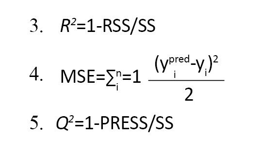
The residual sum of squares (RSS) is the difference between the fitted values and the observed values. It refers to the difference between the observation and their mean. The predictive RSS is the difference between the predictions and the observations.
Results
QSAR-Wrapper-FFNN method
The results obtained from the selection of the most important descriptors by the wrapper method, using the correlation coefficient R and the variance inflation factor VIF, showed that 15 descriptors seemed to be the most appropriate. The calculated VIFs among the values of the selected descriptors were less than five, indicating that multicollinearity between the selected descriptors is acceptable. Supplemental Material 4 shows the VIF values for the selected descriptors and their meanings. To specify the number of hidden neurons required, the procedure detailed above was followed. R (all), MSE (validation), and (validation) criteria were employed for the evaluation of the accuracy of the best model. The best model was chosen according to the minimum MSE (validation) and the maximum R (all), and (validation) [35, 44].
Table 1 shows ten network models developed after the wrapper approach. The results obtained showed that network nine with 45 neurons was the best model with R (all)=0.935, R2train=0.875, Q2=0.871, and MSE (validation)=0.015. The best performance of the model had a topology of 15-[45]-1:15 input nodes, one hidden layer with 45 nodes having the hyperbolic tangent as a transfer function, and one output layer with an identity transfer function. The neural networks were implemented using the neural network toolbox for MATLAB [37].
.jpg)
Figure 2 shows a comparison between the experiment and predicted plasma protein binding values for training, validation, and testing sets. The results showed a close correlation between predicted and observed plasma protein binding.
.jpg)
The FFNN models were trained with the Levenberg-Marquardt backpropagation training function and gradient descent with momentum weight and bias learning function, and the data were partitioned using holdout cross-validation. The difference between R2train and Q2 was equal to 0.004. This difference did not exceed 0.3 indicating the robustness of the model [45].
.jpg)
QSAR-CNN-FFNN method
Regarding the QSAR-CNN-FFNN, the results obtained (Table 2) showed that network seven was the best model with R (all)=0.960, R2train=0.905, Q2=0.964, and MSE (validation)=0.005.
.jpg)
The best performance of the model had a topology of 15-[35]-1:15 input nodes, one hidden layer with 35 nodes having the hyperbolic tangent as a transfer function, and an identity transfer function in the output layer. Figure 3 shows a comparison between experimental and predicted plasma protein binding for training, validation, and testing sets.
.jpg)
The difference between R2train and Q2 is equal to 0.059. This difference is less than 0.3 indicating the robustness of the model [45]. For QSAR-CNN-FFNN, the correlation among each pair of our variables was verified and the results are presented in Supplemental Materials 5. In order to obtain an overview of the correlation structure, a heatmap was used to highlight what is important (Figure 4).

The question now is how much is too much correlation between our neural network inputs. It seems that the general rule of thumb is that if the simple correlation coefficient between two regressors is greater than 0.8 or 0.9, multicollinearity is a serious problem [46]. However, with all the rules of thumb, we get in the statistics, there is nothing black or white about this. In our case, a prediction with a correlation coefficient of 0.8 does not appear fatal for our regression model. We can say that the above results served our theory, where more descriptors are valuable and welcome because we accept that by removing some of the features we are also discarding some of the data we have about the problem.
.jpg)
Discussion
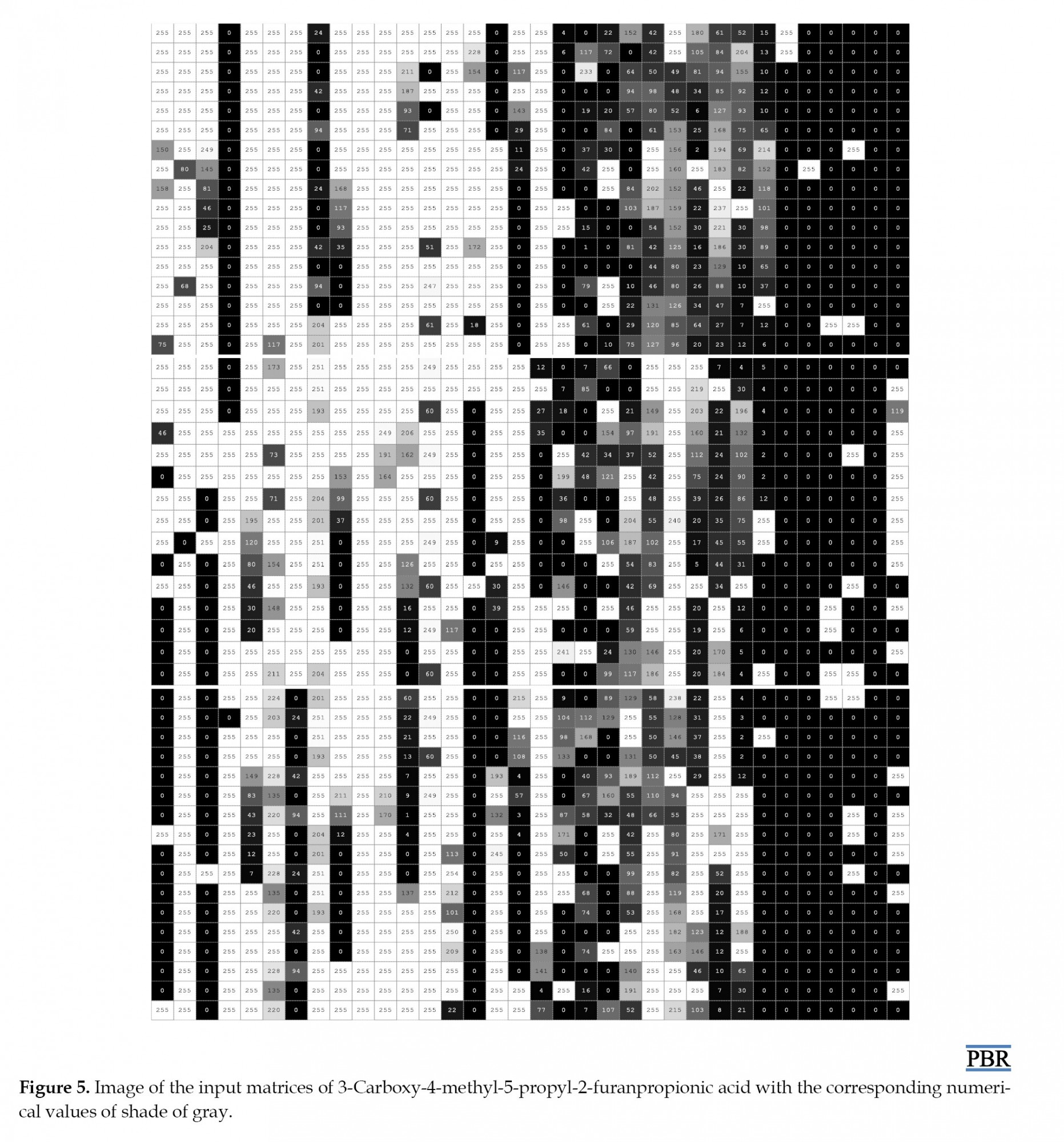
Our results described for the first time the use of CNNs as a feature extraction method in QSAR studies for a set of descriptor matrices instead of local pattern extraction from images. One of the huge favorable circumstances of this method is that it does not take much time (only a few minutes) compared to the wrapper method (which took us days and concentration). It also automatically provides us with features that are the best representation of the non-image input, because in this work, we simply constructed the CNN inputs by resizing the 1666 features to 49×34 matrices. We knew that CNNs are used on data that has spatial features, and the fact that it gave us good features to use is that the CNN used discovered that our data has some sort of spatial features. We wanted to know what this deep CNN actually saw, and how it understands the inputs, we feed them. By visualizing the digital values of our matrices, grayscale images were obtained, giving 255 possible different shades of grey from black to white. Figure 5 shows a sample image of 3-carboxy-4-methyl-5-propyl-2-furanpropionic acid obtained. Numeric values below zero go to zero and those over one go to 255. Values between zero and one are shades of grey, with values between zero and 255. By taking the values of our descriptors and mapping them to the corresponding color suddenly, we can see the structure within our data. We can say that we have made an interface between our data and our brain by visualizing descriptors, in which physical and chemical information about molecules becomes accessible in a new form of fingerprints. They turn into storytellers of molecules secret in just an image.
Comparison of the two models
A statistical evaluation presented in Table 3 was conducted to compare the performance and quality of the predictions by the FFNN of the two models developed for this work. The statistical coefficients of the internal validation for the two models are all acceptable and satisfactory (high R2train, Q2 (validation), R2adjusted and lowest MSE, RMSE, and MAE) and consequently, these models are robust.
.jpg)
The quality of the models was also evaluated in terms of external validation criteria. For the wrapper feature extraction method, a value of Q2>0.5 is considered satisfactory and for the QSAR-CNN feature extraction method, the value of Q2>0.9 is considered excellent [45]. We can say that the two models are distinguished by excellent predictive power.
.jpg)
Comparison between models from the literature
A comparison was made between the few models reported in the literature with those developed in this work for the prediction of the binding of drugs to plasma proteins (Table 4). Yawen Yuan et al. constructed a QSAR model for predicting plasma protein binding based on a large training set comprising more than 5000 compounds and proposed a new strategy for constructing models for different binding levels. Lixia Sun et al. developed QSAR models by six machine learning algorithms with 26 molecular descriptors for predicting the protein-bound fractions of 967 pharmaceuticals.
.jpg)
The neural network model yielded an MAE error of 0.126. Rajnish Kumar et al. presented six machine learning algorithms for QSAR models using a database containing 735 drugs. The model with the artificial neural network gave an MSE train=0.869 and MSE val=0.881. Haiyan Li et al. developed a new method called QSAR Plasma Protein Interaction QSAR Analysis (PPI-QSAR) with a database of 65 antibiotics, providing R2train=0.86 and Q2=0.72. Taravat Ghafourian et al. collected a database of 794 drugs and used four data mining tools; the best model was boosted trees providing an error MAE train=13.25 and an MAE=14.96. Moda Tiago et al. developed a hologram quantitative structure-activity relationship (HQSAR) on a series of 312 drugs, and they obtained a Q2=0.72 and R2=0.91.
.jpg)
We were not interested in evaluating the advantages and disadvantages of these methods because it is quite difficult (each study used different data sets and different modeling approaches) and because the objective of our work was to prove that our new feature selection method is as effective as these old methods. According to these results, the models developed in this work performed as well as these methods.
Applicability domain
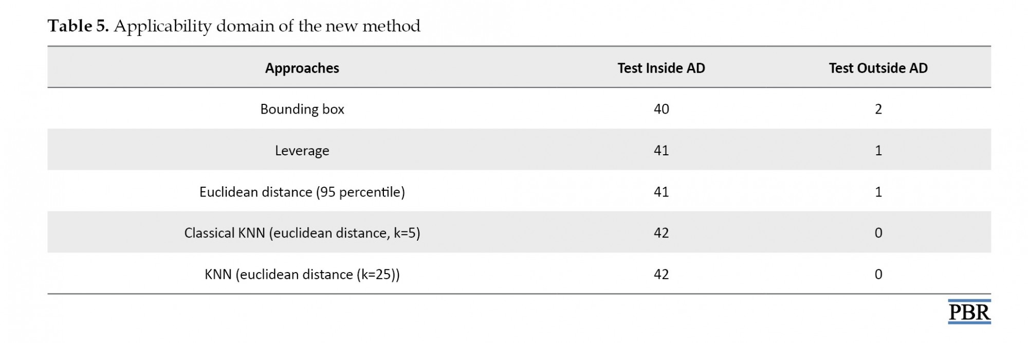
The third principle of the OECD guidelines [47] recommends a defined applicability domain. In this work, the domain of applicability was analyzed with different approaches reported in Table 5.
.jpg)
The algorithm and methodology of the proposed approaches are available in the literature [48]. The number of samples inside the applicability domain varied depending on the method used: the bounding box considered two test samples out of the applicability domain, while leverage and Euclidean distance (95 percentile) identified one test sample out of the domain of applicability as shown in Williams plot (Figure 6).
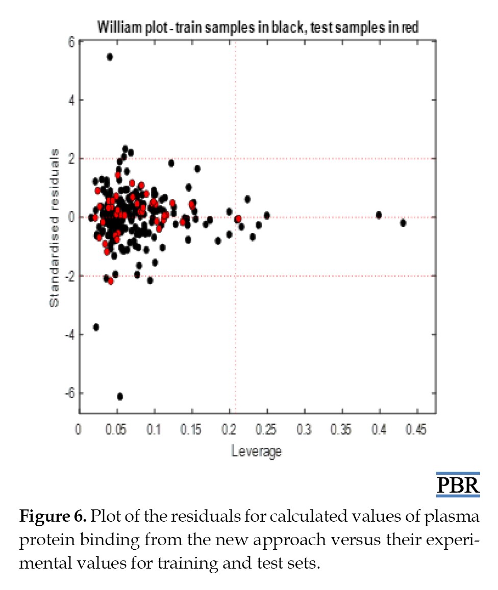
Despite its distance from the other observations, our point is close to the regression fitted line since it has a small residual. Classical KNN (Euclidean distance, k=5) and KNN (Euclidean distance (k=25)) showed none of the test samples out of the applicability domain. These results show that we can use the model to predict plasma protein binding for new compounds that have not been tested.
Conclusion
Two different approaches to feature selection in machine learning were tested. These feature selection strategies were followed to produce inputs, which were used in an FFNN to make predictions. Examination of the estimates of external and internal criteria revealed that the QSAR model developed by the new feature selection method is robust, externally predictive, and distinguished by a good applicability domain. The external accuracy of the validation set was calculated by the Q2 and RMSE, which are equal to 0.945 and 0.085, respectively indicating that the accuracy of NN trained with extracted features from CNNs is slightly better than the accuracy of NN trained with features obtained by the current predictors. This investigation showed that extracting features using CNNs takes less time (only a few minutes) and summarizes much of the information contained in the original features. Contrary to feature selection techniques, we do not have to figure out which features are the best representations of the input, they are learned for us. In the end, according to the OECD principle, we can say that we can use this QSAR-CNN-FFNN model to predict the fraction of plasma protein binding to human plasma for drugs that have not been tested to avoid chemical synthesis and reduce expansive laboratory tests.
Ethical Considerations
Compliance with ethical guidelines
There were no ethical considerations to be considered in this research.
Funding
The authors declare no conflict of interest.
Authors' contributions
Study design: Salah Hanini; Investigation, data collection, and data analysis: Khaouane Affaf; Supervision and Writing–original draft: Samira Ferhat; Writing–review & editing: all authors.
Conflict of interest
The authors declared no conflict of interest.
Acknowledgments
The authors thank the Laboratory of Biomaterial and Transport Phenomena (LBMPT), University of Médéa, for providing the facilities to conduct this study.
References
Building a quantitative structure-activity relationship (QSAR) model, known as in silico model, is an important step in drug discovery. It allows us to avoid chemical synthesis and reduce expansive and tedious laboratory tests [1, 2]. Different QSAR approaches have been developed over the past few years [3-5]. These approaches can determine the quantitative relations between the variation in the values of calculated descriptors and the biological activity of a series of chemical molecules [6]. Thus, once a correlation has been established, it can be used to predict the property or biological activity of new structures [7, 8]. In QSAR studies, selecting a few relevant descriptors from a large number of features is a difficult task. Feature selection techniques are applied to reduce the number of attributes in the dataset by choosing features that will give us better accuracy with fewer data [9-11]. It also reduces the overfitting and the overtraining risk [12]. Feature selection methods can be divided into three categories: filter, wrapper, and embedded methods. Filters are applied independently of the mapping method used. They are executed before the mapping, to reduce the number of descriptors, following some objective criteria [13]. The wrapper techniques are used to select the optimum subset of features based on the error reduction of classifier algorithms. Wrapper methods perform better than filter methods but are more expensive and time-consuming [14]. Features selected with embedded or hybrid methods are sensitive to the structure of the underlying classifiers. Thus, in most cases, the features selected by one embedded method might not be suitable for others [15].
Plasma protein binding plays a key role in drug therapy that affects the pharmacokinetics and pharmacodynamics of the drug, as they are often directly related to the free drug concentration in plasma [16, 17]. In recent years, several QSAR-artificial intelligence models have been developed to predict plasma protein binding, such as support vector machines and their derivatives [18-20], random forest [21], neural networks [22, 23], and gradient-boosting decision trees [24]. In 2017, Sun et al. constructed QSAR models by six machine-learning algorithms with 26 molecular descriptors [25]. Kumar et al. in 2018 presented a systematic approach using a support vector machine, artificial neural network, K-nearest neighbor, probabilistic neural network, partial least square, and linear discriminant analysis to a diverse dataset of 735 drugs [26]. Yuan et al. in 2020 published a global QSAR model for plasma protein binding and developed a novel strategy to construct a robust QSAR model for plasma protein binding prediction [27]. Recently, deep learning algorithms have attracted the attention of scientists and become an important option for pharmaceutical research. Ramsundar et al. presented deep learning techniques for healthcare that efficiently predict drug activity and structure [28]. Wallach et al. introduced AtomNet, known as the first structure-based deep convolutional neural network (CNN), to predict the bioactivity of small molecules for drug discovery applications [29].
In this work, a novel combined methodology based on QSAR, CNN, and a feed-forward neural network (FFNN) was used to predict plasma protein binding for 277 molecules. The CNN, known to be the most popular algorithm for deep learning, was used for feature selection as an alternative to the wrapper method. The FFNN was then used for the prediction of the plasma protein binding from the extracted features.
Material and Metods
In order to predict the plasma protein binding, a methodology based on five steps was used as summarized in Figure 1: (1) data set collection, (2) molecular descriptors generation, (3) selection of relevant descriptors by a wrapper method and a CNN method, (4) FFNN modeling, and (5) validation of models.
.jpg)
Data set collection
The experimental data of protein binding of the 277 drugs used in this study were selected from the pharmacological basis of the therapeutics handbook [30] and the handbook of clinical drug data [31]. Chemical names and experimental protein binding values are presented in Supplemental Material 1.
Molecular descriptors generation
The numerical representation of molecular structure was assessed in terms of molecular descriptors. The SMILES script (simplified molecular-input line-entry system) required to calculate descriptors was extracted from the open-access database PubChem [32]. SMILES is a specification in the form of a line notation describing the structure of chemical species [33]. The SMILES scripts for the 277 drugs were used to generate 1666 descriptors divided into 20 categories: (i) constitutional descriptors, (ii) topological descriptors, (iii) walk and path counts; (iv) connectivity indices; (v) index information; (vi) 2Dautocorrelations; (vii) edge adjacency indices; (viii) burden eigenvalue descriptors; (ix) topological charge indices; (x) eigenvalue-based indices; (xi) Randic molecular profiles; (xii) geometrical descriptors; (xiii) RDF descriptors; (xiv) 3D-MoRSE descriptors; (xv) WHIM descriptors; (xvi) GETAWAY descriptors; (xvii) functional group counts; (xviii) atom-centered fragments; (xix) charge descriptors; and (xx) molecular properties.
All descriptors were obtained through the E-Dragon online programs [34], which is known as the electronic remote version of the well-known software DRAGON developed by the Milano Chemometrics and QSAR Research Group by Prof. R. Todeschini. The name and number of calculated descriptors are reported in Supplemental Material 2.
Selection of relevant descriptors
The selection of the most efficient descriptors, which is an important step in QSAR modeling, was made by two techniques in this work.
Wrapper method
The number of molecular descriptors was reduced by the following procedure [35]:
1) Descriptors having constant values (min=max) were eliminated.
2) Quasi-constant descriptors (1st quartile 25%=2nd quartile 75%) were removed.
3) Descriptors with standard relative deviation RSD<0.05 were deleted.
The three steps above were performed using STATISTICA software [36].
4) Matrices of the pairwise linear correlation between each pair of columns in the input matrices were calculated via MATLAB [37]. In addition, all variables with a correlation coefficient R>0.75 were removed. For more robustness of the model, the variance inflation factor VIF was calculated (Equation 1):

, Where is the squared correlation coefficient of the ith descriptor versus the remaining ones. All the descriptors with VIF>5 were eliminated from the model [38].
5) The remaining descriptors were analyzed by stepwise regression in STATISTICA software [36]. Only 15 descriptors were selected and used as input variables in the FFNN models.
CNN method
CNNs are one of the most popular algorithms for deep learning, and they are mostly used for image classification. Computers do not see an image as an image, but as an array of pixels and the whole process in CNNs depends on it. Therefore, we provided our CNN network with previously digitalized data as input. Because for deep learning, in image classification, we do not have to understand which features are the best representations of the object, they are taught to us.
In our approach, the 1666 descriptors calculated with E-DRAGON were transformed for each drug into matrices of size 49-by-34-by-1 dimension in MATLAB because CNN requires matrices as inputs [39]. The latest features learned from the CNN layers were flattened out and passed through an FFNN to make predictions.
FFNN modeling
QSAR-wrapper-FFNN
The selected descriptors by the wrapper technique were set as input in an FFNN. So far, there is no clear answer to specify the number of hidden neurons required for a modeling task and it remains an open question. Different approaches are discovering this number, explained in detail in reviews, including methods of selecting the number of hidden nodes in the artificial neural networks review [40]. To decide the number of neurons in the hidden layer, the procedure summarized below was used [41]:
1) In the beginning, only a few hidden neurons (five) were used.
2) The network was trained until the mean square error no longer seemed to improve.
3) At this moment, a few (five) neurons were added to the hidden layer, each with randomly initialized weights, and resumed training.
4) The previous two steps were repeated until a termination criterion has been satisfied.
The mathematical equation of the model, for the prediction of protein binding, is shown below (Equation 2):

x i (i=1…p) is the input that corresponds to the number of data included in the training of the ANN, I from 1 to 15, wij (i=1…p, j=1…k) weight from input to hidden layer, b j (j=1…k) are biases of the neurons in the hidden layer, k=45 for Wrapper method, w2j (j=1…k) are weights from the hidden to the output layer, b is the bias of the output neuron, and fb is the output.
QSAR-CNN-FFNN
CNN is a powerful machine learning technique. Training a CNN requires a large collection of diverse data, which is not an easy task [42]. However, there is an easy way, we can use a pre-trained CNN, which saves a huge amount of time and effort because fine-tuning a network with transfer learning is usually much faster and easier than training a network from scratch [43]. In this work, transfer learning using the ALEXNET CNN was applied to perform feature extraction and then feature reduction with adjustment in the last six layers by new ones. The CNN model was used to extract representative feature vectors from the penultimate fully connected layer, and then these ’’deep features’’ were used for training an FFNN. The choice of dimension 15 for the feature reduction is to perform a comparison with the features selected by wrapper methods. The details of the 22 layers are reported in Supplemental Material 3. To train the network, holdout cross-validation was used to divide the data randomly 70% for training, 15% for validation, and 15% for testing.
Validation of the models
To determine both the generalizability and the actual predictive capacity of the QSAR models, internal and external validation criteria were used for the validation of the models. The statistical parameters used in our study to check the performance of the models were the coefficient of determination (R2), the correlation coefficient (R), the predictive squared correlation coefficient (Q2), and the mean squared error values (MSE) (Equations 3-5):

The residual sum of squares (RSS) is the difference between the fitted values and the observed values. It refers to the difference between the observation and their mean. The predictive RSS is the difference between the predictions and the observations.
Results
QSAR-Wrapper-FFNN method
The results obtained from the selection of the most important descriptors by the wrapper method, using the correlation coefficient R and the variance inflation factor VIF, showed that 15 descriptors seemed to be the most appropriate. The calculated VIFs among the values of the selected descriptors were less than five, indicating that multicollinearity between the selected descriptors is acceptable. Supplemental Material 4 shows the VIF values for the selected descriptors and their meanings. To specify the number of hidden neurons required, the procedure detailed above was followed. R (all), MSE (validation), and (validation) criteria were employed for the evaluation of the accuracy of the best model. The best model was chosen according to the minimum MSE (validation) and the maximum R (all), and (validation) [35, 44].
Table 1 shows ten network models developed after the wrapper approach. The results obtained showed that network nine with 45 neurons was the best model with R (all)=0.935, R2train=0.875, Q2=0.871, and MSE (validation)=0.015. The best performance of the model had a topology of 15-[45]-1:15 input nodes, one hidden layer with 45 nodes having the hyperbolic tangent as a transfer function, and one output layer with an identity transfer function. The neural networks were implemented using the neural network toolbox for MATLAB [37].
.jpg)
Figure 2 shows a comparison between the experiment and predicted plasma protein binding values for training, validation, and testing sets. The results showed a close correlation between predicted and observed plasma protein binding.
.jpg)
The FFNN models were trained with the Levenberg-Marquardt backpropagation training function and gradient descent with momentum weight and bias learning function, and the data were partitioned using holdout cross-validation. The difference between R2train and Q2 was equal to 0.004. This difference did not exceed 0.3 indicating the robustness of the model [45].
.jpg)
QSAR-CNN-FFNN method
Regarding the QSAR-CNN-FFNN, the results obtained (Table 2) showed that network seven was the best model with R (all)=0.960, R2train=0.905, Q2=0.964, and MSE (validation)=0.005.
.jpg)
The best performance of the model had a topology of 15-[35]-1:15 input nodes, one hidden layer with 35 nodes having the hyperbolic tangent as a transfer function, and an identity transfer function in the output layer. Figure 3 shows a comparison between experimental and predicted plasma protein binding for training, validation, and testing sets.
.jpg)
The difference between R2train and Q2 is equal to 0.059. This difference is less than 0.3 indicating the robustness of the model [45]. For QSAR-CNN-FFNN, the correlation among each pair of our variables was verified and the results are presented in Supplemental Materials 5. In order to obtain an overview of the correlation structure, a heatmap was used to highlight what is important (Figure 4).

The question now is how much is too much correlation between our neural network inputs. It seems that the general rule of thumb is that if the simple correlation coefficient between two regressors is greater than 0.8 or 0.9, multicollinearity is a serious problem [46]. However, with all the rules of thumb, we get in the statistics, there is nothing black or white about this. In our case, a prediction with a correlation coefficient of 0.8 does not appear fatal for our regression model. We can say that the above results served our theory, where more descriptors are valuable and welcome because we accept that by removing some of the features we are also discarding some of the data we have about the problem.
.jpg)
Discussion
Our results described for the first time the use of CNNs as a feature extraction method in QSAR studies for a set of descriptor matrices instead of local pattern extraction from images. One of the huge favorable circumstances of this method is that it does not take much time (only a few minutes) compared to the wrapper method (which took us days and concentration). It also automatically provides us with features that are the best representation of the non-image input, because in this work, we simply constructed the CNN inputs by resizing the 1666 features to 49×34 matrices. We knew that CNNs are used on data that has spatial features, and the fact that it gave us good features to use is that the CNN used discovered that our data has some sort of spatial features. We wanted to know what this deep CNN actually saw, and how it understands the inputs, we feed them. By visualizing the digital values of our matrices, grayscale images were obtained, giving 255 possible different shades of grey from black to white. Figure 5 shows a sample image of 3-carboxy-4-methyl-5-propyl-2-furanpropionic acid obtained. Numeric values below zero go to zero and those over one go to 255. Values between zero and one are shades of grey, with values between zero and 255. By taking the values of our descriptors and mapping them to the corresponding color suddenly, we can see the structure within our data. We can say that we have made an interface between our data and our brain by visualizing descriptors, in which physical and chemical information about molecules becomes accessible in a new form of fingerprints. They turn into storytellers of molecules secret in just an image.

Comparison of the two models
A statistical evaluation presented in Table 3 was conducted to compare the performance and quality of the predictions by the FFNN of the two models developed for this work. The statistical coefficients of the internal validation for the two models are all acceptable and satisfactory (high R2train, Q2 (validation), R2adjusted and lowest MSE, RMSE, and MAE) and consequently, these models are robust.
.jpg)
The quality of the models was also evaluated in terms of external validation criteria. For the wrapper feature extraction method, a value of Q2>0.5 is considered satisfactory and for the QSAR-CNN feature extraction method, the value of Q2>0.9 is considered excellent [45]. We can say that the two models are distinguished by excellent predictive power.
.jpg)
Comparison between models from the literature
A comparison was made between the few models reported in the literature with those developed in this work for the prediction of the binding of drugs to plasma proteins (Table 4). Yawen Yuan et al. constructed a QSAR model for predicting plasma protein binding based on a large training set comprising more than 5000 compounds and proposed a new strategy for constructing models for different binding levels. Lixia Sun et al. developed QSAR models by six machine learning algorithms with 26 molecular descriptors for predicting the protein-bound fractions of 967 pharmaceuticals.
.jpg)
The neural network model yielded an MAE error of 0.126. Rajnish Kumar et al. presented six machine learning algorithms for QSAR models using a database containing 735 drugs. The model with the artificial neural network gave an MSE train=0.869 and MSE val=0.881. Haiyan Li et al. developed a new method called QSAR Plasma Protein Interaction QSAR Analysis (PPI-QSAR) with a database of 65 antibiotics, providing R2train=0.86 and Q2=0.72. Taravat Ghafourian et al. collected a database of 794 drugs and used four data mining tools; the best model was boosted trees providing an error MAE train=13.25 and an MAE=14.96. Moda Tiago et al. developed a hologram quantitative structure-activity relationship (HQSAR) on a series of 312 drugs, and they obtained a Q2=0.72 and R2=0.91.
.jpg)
We were not interested in evaluating the advantages and disadvantages of these methods because it is quite difficult (each study used different data sets and different modeling approaches) and because the objective of our work was to prove that our new feature selection method is as effective as these old methods. According to these results, the models developed in this work performed as well as these methods.
Applicability domain
The third principle of the OECD guidelines [47] recommends a defined applicability domain. In this work, the domain of applicability was analyzed with different approaches reported in Table 5.
.jpg)
The algorithm and methodology of the proposed approaches are available in the literature [48]. The number of samples inside the applicability domain varied depending on the method used: the bounding box considered two test samples out of the applicability domain, while leverage and Euclidean distance (95 percentile) identified one test sample out of the domain of applicability as shown in Williams plot (Figure 6).

Despite its distance from the other observations, our point is close to the regression fitted line since it has a small residual. Classical KNN (Euclidean distance, k=5) and KNN (Euclidean distance (k=25)) showed none of the test samples out of the applicability domain. These results show that we can use the model to predict plasma protein binding for new compounds that have not been tested.

Conclusion
Two different approaches to feature selection in machine learning were tested. These feature selection strategies were followed to produce inputs, which were used in an FFNN to make predictions. Examination of the estimates of external and internal criteria revealed that the QSAR model developed by the new feature selection method is robust, externally predictive, and distinguished by a good applicability domain. The external accuracy of the validation set was calculated by the Q2 and RMSE, which are equal to 0.945 and 0.085, respectively indicating that the accuracy of NN trained with extracted features from CNNs is slightly better than the accuracy of NN trained with features obtained by the current predictors. This investigation showed that extracting features using CNNs takes less time (only a few minutes) and summarizes much of the information contained in the original features. Contrary to feature selection techniques, we do not have to figure out which features are the best representations of the input, they are learned for us. In the end, according to the OECD principle, we can say that we can use this QSAR-CNN-FFNN model to predict the fraction of plasma protein binding to human plasma for drugs that have not been tested to avoid chemical synthesis and reduce expansive laboratory tests.
Ethical Considerations
Compliance with ethical guidelines
There were no ethical considerations to be considered in this research.
Funding
The authors declare no conflict of interest.
Authors' contributions
Study design: Salah Hanini; Investigation, data collection, and data analysis: Khaouane Affaf; Supervision and Writing–original draft: Samira Ferhat; Writing–review & editing: all authors.
Conflict of interest
The authors declared no conflict of interest.
Acknowledgments
The authors thank the Laboratory of Biomaterial and Transport Phenomena (LBMPT), University of Médéa, for providing the facilities to conduct this study.
References
- Sliwoski G, Kothiwale S, Meiler J, Lowe EW Jr. Computational methods in drug discovery. Pharmacol Rev. 2013; 66(1):334-95. [DOI:10.1124/pr.112.007336] [PMID] [PMCID]
- Lin X, Li X, Lin X. A review on applications of computational methods in drug screening and design. Molecules. 2020; 25(6):1375. [DOI:10.3390/molecules25061375] [PMID] [PMCID]
- Kubinyi H. QSAR and 3D QSAR in drug design Part 1: methodology. Drug Discovery Today. 1997; 2(11):457-67. [DOI:10.1016/S1359-6446(97)01084-2]
- Khan MT. Predictions of the ADMET properties of candidate drug molecules utilizing different QSAR/QSPR modelling approaches. Curr Drug Metab. 2010; 11:285-95. [DOI:10.2174/138920010791514306] [PMID]
- Zhang L, Tan J, Han D, Zhu H. From machine learning to deep learning: Progress in machine intelligence for rational drug discovery. Drug Discov Today. 2017; 22(11):1680-5. [DOI:10.1016/j.drudis.2017.08.010] [PMID]
- Rasulev BF, Abdullaev ND, Syrov VN, Leszczynski J. A quantitative structure‐activity relationship (QSAR) study of the antioxidant activity of flavonoids. QSAR Comb Sci. 2005; 24:1056-65. [DOI:10.1002/qsar.200430013]
- Nirmalakhandan N, Speece RE. ES & T critical review: Structure-activity relationships. Quantitative techniques for predicting the behavior of chemicals in the ecosystem. Environ Sci Technol. 1988; 22:606-15. [DOI:10.1021/es00171a002]
- Grover M, Singh B, Bakshi M, Singh S. Quantitative structure-property relationships in pharmaceutical research-Part 1. Pharm Sci Technol. 2000; 3(2):50-57. [DOI:10.1016/S1461-5347(99)00214-X]
- Hira ZM, Gillies DF. A review of feature selection and feature extraction methods applied on microarray data. Adv Bioinformatics. 2015; 2015:198363. [DOI:10.1155/2015/198363] [PMID] [PMCID]
- Langley P. Selection of relevant features in machine learning. Palo Alto: Institute for the Study of Learning and Expertise; 1994. [DOI:10.21236/ADA292575]
- Dash M, Liu H. Feature selection for classification. Intell Data Anal. 1997; 1(1-4):131-56. [DOI:10.1016/S1088-467X(97)00008-5]
- Tetko IV, Livingstone DJ, Luik AI. Neural network studies. 1. Comparison of overfitting and overtraining. J Chem Inf Comput Sci. 1995:35(5):826–33. [DOI:10.1021/ci00027a006]
- Dudek AZ, Arodz T, Gálvez J. Computational methods in developing quantitative structure-activity relationships (QSAR): A review. Comb Chem High Throughput Screen. 2006; 9(3):213-28. [DOI:10.2174/138620706776055539] [PMID]
- Ghasemi F, Mehridehnavi A, Pérez-Garrido A, Pérez-Sánchez H. Neural network and deep-learning algorithms used in QSAR studies: Merits and drawbacks. Drug Discov Today. 2018; 23(10):1784-90. [DOI:10.1016/j.drudis.2018.06.016] [PMID]
- Danishuddin, Khan AU. Descriptors and their selection methods in QSAR analysis: Paradigm for drug design. Drug Discov Today. 2016; 21(8):1291-302. [DOI:10.1016/j.drudis.2016.06.013] [PMID]
- Bohnert T, Gan LS. Plasma protein binding: From discovery to development. J Pharm Sci. 2013; 102(9):2953-94. [DOI:10.1002/jps.23614] [PMID]
- Trainor GL. The importance of plasma protein binding in drug discovery. Expert Opin Drug Discov. 2007; 2(1):51-64. [DOI:10.1517/17460441.2.1.51] [PMID]
- Zsila F, Bikadi Z, Malik D, Hari P, Pechan I, Berces A, et al. Evaluation of drug-human serum albumin binding interactions with support vector machine aided online automated docking. Bioinformatics. 2011; 27(13):1806-13. [DOI:10.1093/bioinformatics/btr284] [PMID]
- Guo Y, Yu L, Wen Z, Li M. Using support vector machine combined with auto covariance to predict protein-protein interactions from protein sequences. Nucleic Acids Res. 2008; 36(9):3025-30. [DOI:10.1093/nar/gkn159] [PMID] [PMCID]
- Zhao C, Zhang H, Zhang X, Zhang R, Luan F, Liu M, et al. Prediction of milk/plasma drug concentration (M/P) ratio using support vector machine (SVM) method. Pharmaceutical Res. 2006; 23(1):41-8. [DOI:10.1007/s11095-005-8716-4] [PMID]
- Ghafourian T, Amin Z. QSAR models for the prediction of plasma protein binding. Bioimpacts. 2013; 3(1):21-7. [DOI:10.5681/bi.2013.011] [PMID] [PMCID]
- Fu X, Wang G, Gao J, Zhan S, Liang W. Prediction of plasma protein binding of cephalosporins using an artificial neural network. Pharmazie. 2007; 62(2):157-8. [PMID]
- Turner JV, Maddalena DJ, Cutler DJ. Pharmacokinetic parameter prediction from drug structure using artificial neural networks. Int J Pharm. 2004; 270(1-2):209-19. [DOI:10.1016/j.ijpharm.2003.10.011] [PMID]
- Deng L, Sui Y, Zhang J. XGBPRH: Prediction of binding hot spots at protein-RNA interfaces utilizing extreme gradient boosting. Genes. 2019; 10(3):242. [DOI:10.3390/genes10030242] [PMID] [PMCID]
- Sun L, Yang H, Li J, Wang T, Li W, Liu G, et al. In silico prediction of compounds binding to human plasma proteins by QSAR models. Chem Med Chem. 2018; 13(6):572-81. [DOI:10.1002/cmdc.201700582] [PMID]
- Kumar R, Sharma A, Siddiqui MH, Tiwari RK. Prediction of drug-plasma protein binding using artificial intelligence based algorithms. Comb Chem High Throughput Screen. 2018; 21(1):57-64. [DOI:10.2174/1386207321666171218121557] [PMID]
- Yuan Y, Chang S, Zhang Z, Li Z, Li S, Xie P, et al. A novel strategy for prediction of human plasma protein binding using machine learning techniques. Chemometr Intell Lab Syst. 2020; 199:103962. [DOI:10.1016/j.chemolab.2020.103962]
- Altae-Tran H, Ramsundar B, Pappu AS, Pande V. Low data drug discovery with one-shot learning. ACS Cent Sci. 2017; 3(4):283-93. [DOI:10.1021/acscentsci.6b00367] [PMID] [PMCID]
- Wallach I, Dzamba M, Heifets A. AtomNet: A deep convolutional neural network for bioactivity prediction in structure-based drug discovery. arXi v:1510.02855v1. 2015; 1-11. [DOI:10.48550/arXiv.1510.02855]
- Brunton L, Lazo J, Parker K. Goodman & Gilman’s the pharmacological basis of therapeutics. New York: McGraw Hill Professional; 2005. [Link]
- Troutman WG. Handbook of clinical drug data. New York: McGraw-Hill; 2002. [Link]
- PubChem. National Institutes of Health (NIH). https://pubchemdocs.ncbi.nlm.nih.gov/
- Weininger D. SMILES, a chemical language and information system. 1. Introduction to methodology and encoding rules. J Chem Inf Comput Sci. 1988; 28(1):31–6. [DOI:10.1021/ci00057a005]
- Virtual Computational Chemistry Laboratory (VCCLAB). http://www.vcclab.org/
- Hamadache M, Benkortbi O, Hanini S, Amrane A, Khaouane L, Moussa CS. A quantitative structure activity relationship for acute oral toxicity of pesticides on rats: Validation, domain of application and prediction. J Hazard Mater. 2016; 303:28-40. [DOI:10.1016/j.jhazmat.2015.09.021] [PMID]
- Stat Soft Inc. STATISTICA, Version 8 [Internet]. 2007 [Updated November 2022]. Available from: [Link]
- Math Works MATLAB R2019b. MathWorks, Inc. [Internet]. 2022 [Updated November 2022]. Available from: [Link]
- Akinwande MO, Dikko HG, Samson A. Variance inflation factor: As a condition for the inclusion of suppressor variable (s) in regression analysis. “Open J Stat. 2015; 5:754-67. [DOI:10.4236/ojs.2015.57075]
- Bazgir O, Zhang R, Dhruba SR, Rahman R, Ghosh S, Pal R. Representation of features as images with neighborhood dependencies for compatibility with convolutional neural networks. Nat Commun. 2020; 11:4391. [DOI:10.1038/s41467-020-18197-y] [PMID] [PMCID]
- Panchal FS, Panchal M. Review on methods of selecting number of hidden nodes in artificial neural network. Int J Comput Sci Mob Computing. 2014; 3(11):455-64. [Link]
- Kubat M. An introduction to machine learning. Cham: Springer; 2017. [DOI:10.1007/978-3-319-63913-0]
- Tajbakhsh N, Shin JY, Gurudu SR, Hurst RT, Kendall CB, Gotway MB, et al. Convolutional neural networks for medical image analysis: Full training or fine tuning? IEEE Trans Med Imaging. 2016; 35(5):1299-312 [DOI:10.1109/TMI.2016.2535302] [PMID]
- Schwarz M, Schulz H, Behnke S. RGB-D object recognition and pose estimation based on pre-trained convolutional neural network features. Paper presented at: 2015 IEEE International Conference on Robotics and Automation (ICRA). 26-30 May 2015; Seattle, USA. [DOI:10.1109/ICRA.2015.7139363]
- Bitam S, Hamadache M, Hanini S. QSAR model for prediction of the therapeutic potency of N-benzylpiperidine derivatives as AChE inhibitors. SAR QSAR Environ Res. 2017; 28(6):471-49. [DOI:10.1080/1062936X.2017.1331467] [PMID]
- Eriksson L, Jaworska J, Worth AP, Cronin MT, McDowell RM, Gramatica P. Methods for reliability and uncertainty assessment and for applicability evaluations of classification- and regression-based QSARs. Environ Health Perspect. 2003; 111(10):1361-75. [DOI:10.1289/ehp.5758] [PMID] [PMCID]
- Midi H, Sarkar SK, Rana S. Collinearity diagnostics of binary logistic regression model. J Interdiscip Math. 2010; 13:253-67. [DOI:10.1080/09720502.2010.10700699]
- Organisation for Economic Co-operation and Development (OECD). Guidance document on the validation of (quantitative) structure-activity relationship [(Q)SAR] models., Paris: OECD Publishing; 2014. [Link]
- Roy K, Kar S, Ambure P. On a simple approach for determining applicability domain of QSAR models. Chemom Intell Lab Syst. 2015; 145:22-9. [DOI:10.1016/j.chemolab.2015.04.013]
- Li H, Chen Z, Xu X, Sui X, Guo T, Liu W, et al. Predicting human plasma protein binding of drugs using plasma protein interaction QSAR analysis (PPI-QSAR). Biopharm Drug Dispos. 2011; 32(6):333-42. [DOI:10.1002/bdd.762] [PMID]
- Moda TL, Montanari CA, Andricopulo AD. In silico prediction of human plasma protein binding using hologram QSAR. Lett Drug Des Discov. 2007; 4(7):502-9. [DOI:10.2174/157018007781788480]
Type of Study: Original Research |
Subject:
Mollecular Modeling
| Rights and permissions | |
 |
This work is licensed under a Creative Commons Attribution-NonCommercial 4.0 International License. |


